Using Indexing to detect regions of interest and extracting their shape features with a FITS file.
In this tutorial you will learn: * How to use the Indexing Class. * Converting FITS into data cubes. * Visualizing data.
The Indexing Algorithm is a class that takes a data cube, specifically an image and returns: * the cube slices * region of interest tables for each scale analyzed * segmentated images
If you have a FITS you can convert it to data with the functions that ACALIB has prepared for it. In this tutorial we will use ‘example.fits’ as our FITS archive.
First we must import our library
import acalib
We have a FITS file so it must be converted to be used on the library.
To handle the FITS acalib counts with a series of functions and classes, one of them is load_fits(), and the container class. We will use these to convert our file into a NDDATA list, so our indexing class can read it.
c = acalib.Container()
c.load_fits('/home/AtoMQuarK/LIRAE/fits/example.fits')
INFO: Processing HDU 0 (Image) [acalib.io.fits]
INFO: 4D data detected: assuming RA-DEC-FREQ-STOKES (like CASA-generated ones), and dropping STOKES [acalib.io.fits]
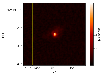
For indexing we need only the primary data cube, so we use a function called primary from the acalib Container.
cube = c.primary
Now we can run the indexing Class, we can configure its precision and number of samples too.
idx=acalib.Indexing()
idx.config['PRECISION']=0.01
idx.config['SAMPLES']=int(100)
cont=idx.run(cube)
INFO: overwriting NDData's current wcs with specified wcs. [astropy.nddata.nddata]
Indexing returns the tables with the regions of interest, here you can see the table.
for i in range(len(cont.tables)):
    print(cont.tables[i])
  CentroidRa   CentroidDec  MajorAxisLength ... MinIntensity AverageIntensity
------------- ------------- --------------- ... ------------ ----------------
119.376367615 113.288840263   41.7786837299 ...      0.01555         0.593364
49.7119565217 118.364130435   17.5783827847 ...  -0.00521045        0.0494876
         62.0         100.0   12.0058982555 ...   -0.0259817        0.0156168
73.5724770642 130.609174312   31.9413760412 ...   -0.0512585        0.0119501
71.7798742138 81.6981132075   15.3993338417 ...   -0.0464124       0.00651135
 130.67835015 101.781554257   143.624244379 ...   -0.0512814        0.0111981
         95.5          41.0   14.7862823705 ...  -0.00730038         0.030496
132.794117647 164.173796791   31.5736614836 ...   -0.0484251         0.022494
        155.0         138.0   14.0543651531 ...   -0.0510979       0.00134066
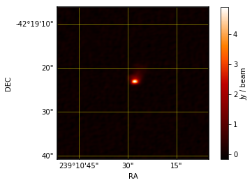
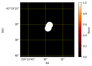
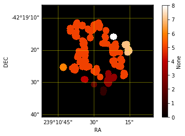
It also returns the segmentated images.
acalib.visualize(acalib.moment0(cont.primary))
Here we visualize the segmentated images
for i in range(1,len(cont.images)):
    acalib.visualize(cont.images[i])
With this you learned how to use the Indexing Class and visualize its information, and how to manipulate the data from a FITS file. Feel free to use these functions as you need!